In the last part of this AMDIS discussion, the setting up and running of a simple analysis was discussed. However, to take full advantage of AMDIS it is far better to make use not only of the mass spectral information, but also the retention time data. In Part 2 of the “Setting Up and Running a Deconvolution and Target Analysis”, we will discuss setting up and using the retention information and briefly discuss the various parameters that can be set by the user.
The comparison of an extracted component with a library mass spectrum can often be fully decisive of the identity. There are some compounds where the spectrum is so nearly unique that the chance for misidentification is very low. Many pesticides are in this category as are compounds such as the chemical warfare agent sulfur mustard. However, for the majority of chemical compounds, the spectral information alone may not be sufficient to distinguish between many similar compounds. Specific cases of this include important classes of compounds such as essential oil components — terpenes, trimethylsilyl derivatives of many polar organic compounds, hydrocarbons and compounds that have very simple mass spectra such as many amines. For many of these compounds the use of retention information is especially valuable. AMDIS uses (by default) the normal Kovats retention index for temperature ramped columns as discussed by van den Dool and Kratz. Here the linear hydrocarbons are assigned a retention index equal to 100*Carbon Number and the retention index of a component is defined in terms of the elution times of the linear standards eluting before (Tb) and after (Ta) and their corresponding retention indices (Rib and RIa) and the time (Tc)of the component:
RIc =Rib+( RIa -(RIb)*( Tc-Tb)/(Tb-Ta)
For most systems, the stability of the column is sufficient so that a calibration file resulting from the injection of a mixture of linear hydrocarbons, typically from octane(C8) to tetracosane (C24), is run under the same chromatographic conditions as the experiments. If late eluting compounds are also of interest the calibration mixture should contain the hydrocarbons up to elution times beyond the last compound of interest. The calculation of the RI for the components is done automatically by AMDIS and the results of the RI calculation compared to the library value much as is done for the mass spectrum.

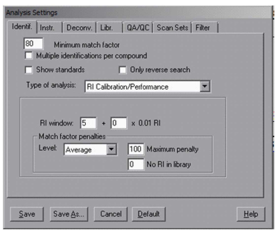
AMDIS has a special library that contains only the retention index standards — hydrocarbons (a sample of such a library is in the distribution) — and if desired any other compounds that are used for routine quality control. This library is used to analyse the data file of the calibration compounds. To have AMDIS create a calibration file for use with your data, you need (1) a data file of the hydrocarbons and (2) the hydrocarbon library — the standards library are named *.csl (unlike the target libraries which are *.msl). The result of the calibration is kept in a file *.cal. The location and name of the file is the user’s choice – note, you assign the name to the file but it does not need to exist prior to the analysis. To analyze the calibration data file, it must first be loaded and then the analysis type is set to “RI Calibration/Performance”. For calibration analysis it is best to use high minimum match factors (80 or 90) and leave unchecked “Multiple identifications per compound”. A typical Analysis Setting “Ident.” (Identification) screen will look like Figure 1. In addition, it is necessary to specify a library and as noted above a calibration file. This is all done in the ” Libr.” (Library) tab. The Calibration/Standards Library needs to be selected only once. The RI Calibration Data file may be changed as new calibration runs are made. The data file will be analyzed and the calibration compounds found will be used to establish the calibration table that is used by the program to convert retention time into retention index.
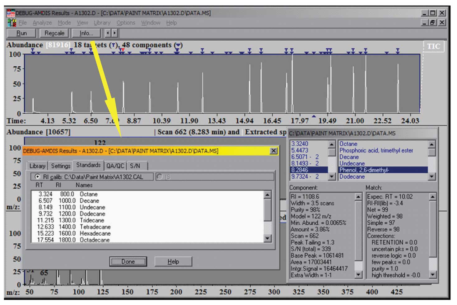
Typically, QA/QC compounds, such as the Grob mixture, are also in a QA calibration experiment. Spectra and retention indices for these compounds are also placed in the CSL library. The results of the analysis are both the normal display showing the data found and the match factors, as well as the calibration file, which can be seen using the Info button. The results of a calibration analysis are shown in Figure 2 along with the information from the Info button.
Once a calibration has been established, we can use the retention index information to aid in the analysis of the data. The role of retention data can be critical in the identification of species where many different chemicals have similar spectra, however, the retention index data must be included in the library for this option to be useful. In cases such as those mentioned above the retention information can reduce the number of identifications for a single component from 5 to 10 to just 1.
Using the Retention Penalty
To make use of the RI data for an analysis, the “Type of Analysis” must be set to “Use Retention Index Data”. Once this is done you will have to decide on the RI window and the level of the match factor penalties. The RI data can only be used to reduce the mass spectral match factor, it will not increase it. The RI penalty works by looking at the absolute difference of the measured RI for a component and the library RI of the tentative identification (RIdiff =| RIlib – RImeas|). If RIdiff is less than the value specified in the RI window box, then there is no penalty. Once RIdiff is greater than the window, a penalty is applied that is proportional to the size of the window and the Level set for the match factor penalties. The Level choices are Weak, Average, Strong, Very Strong and Infinite. These choices correspond to a penalty of 1,5,10,20 and 1000 match factor points per window (beyond the initial window). To illustrate this, if the window is set to 5, the penalty level to Strong and RIdiff is 9 — the match factor penalty will be 8. The first window of difference (5 in this case) is without penalty, the difference between RIdiff and the RI window is thus 4 and the strong penalty is assessed in terms of this value and the penalty level (4/5*10).
This can be expressed as an equation:
RI Penalty = ( [ (RIdiff –RI Window)/(RI Window) ] – 1 )* Level Factor
Where Level Factor is as noted above (1,5,10,20,1000), and the -1 accounts for the lack of penalty if the RIdiffis within the RI Window. Note that RI Penalty only applies if it is greater than 0.
The choice of the RI window and level can be important. For example, if there are a number of isomers that are close in retention index in the target library, then a small window (for example 2) with an Average penalty level could differentiate between the isomers. If however the experimental matrix is variable enough that there are retention shifts from run to run, a larger RI window may be necessary to avoid penalty of good identifications. The cut-off conditions used in some pesticide analysis where only very narrow RI windows are allowed can be created by choosing the Infinite Level. Here, if the measured RI is outside of the RI window by even 1/10 of the window the match is penalized by 100 points.

It is also possible to allow the RI window to increase as RI increases and to penalize a compound if there is no RI in the library. The effect of this latter action is to require spectra that do not have RI data to have a higher match factor than spectra that do have RI data. Ideally all spectra in the library have RI data associated with them and the penalty is set to 0. Finally, it is possible to change the maximum penalty that is applied. The Minimum match factor is the lowest value of a match factor that will be reported as a target. If the Minimum match factor is 70, then it will not matter if the Maximum penalty is 30 or 100, the same set of data will be reported, but if Minimum match factor is 60, then data that would have had a penalty of 50 points because RI will only be penalized a maximum of 30 in the case where the Maximum penalty is 30 and may be still reported if the mass spectral match factor was very good.
Setting Deconvolution Parameters
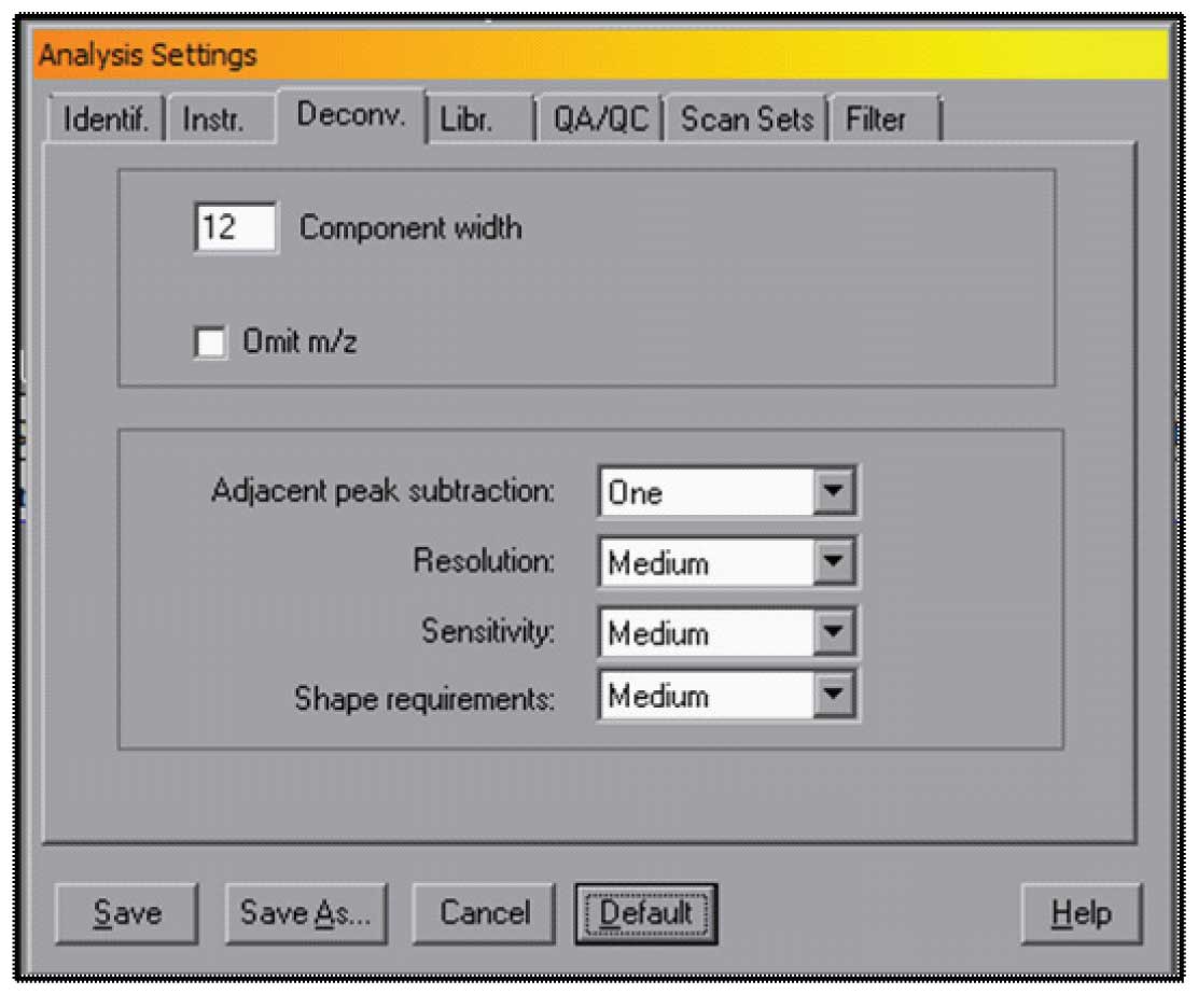
The choice of the retention window and minimum match factor are very important, but there are other factors that can be set in AMDIS that will allow for more control over the way the data is analysed. The most important of these are found in the Analyze Settings Tabbed Dialog under “Deconv.” – Deconvloution. There are a set of Default parameters that will work for a wide variety of data. These are shown in Figure 3, and can be accessed by selecting the Default button in this window.
The settings are Component width which is the number of scans from the maximum of a component that AMDIS will go before stopping and extracting a spectrum. The assumption that is made with this default condition is that a normal peak (meaning one that is not strongly affected by the column) will have a full width of about 6-10 scans. The value of 12 will allow for almost a factor of two greater width. If you have strongly tailing peaks, it is may be valuable to set this value to a larger number. The maximum value 32 (in older versions of AMDIS the maximum was 20). AMDIS will calculate better areas of the peaks with long tails if you use a larger number, but it can slightly slow down the program.
The Settings in the lower box are Adjacent peak subtraction (None, One, Two), Resolution (Low, Medium, High), Sensitivity (Very Low, Low, Medium, High, Very High), Shape Requirements (Low, Medium, High). These parameters do interact to some degree, but all are related to how sensitive AMDIS is to low signals and how you may want to differentiate low signals from noise.

Adjacent peak subtraction allows the program to use or not use a second peak in the deconvolution of a component. In some cases the best spectrum for a target can only be extracted when a very close nearby peak is explicitly subtracted – however in many cases even very closely coeluting components can be separated without the subtraction. The default is one adjacent peak, and under almost all conditions this is sufficient. At all times the program will report the model peak used for the deconvolution and when a subtraction is made the report is “Model = 100 m/z (137)” meaning that the ion at m/z 100 was used as the model peak, but there was an explicit subtraction of the ions associated with the other model – 137.
Resolution sets how close the maximum of two ion profiles can be and still be seen as distinct peaks. To some extent this will depend upon how large the signal is, two very strong closely eluting peaks can be resolved better than two very weak peaks with the same separation. Typically, with medium resolution it is possible to extract components that are ½ a scan or more apart.
Sensitivity sets how small a signal (in terms of signal-to-noise units) is declared to be a signal and not noise. Between very low and very high the number of components can change by over a factor of 3, but except for very weak target molecule signals, the number of identified components will not change. For use in pesticide analysis, it may be useful to use high or even very high sensitivity, but only for target searches. For metabolic studies or any attempt to locate components for which the initial target spectra are not known, lower sensitivities are generally better.
Shape requirements determine how closely the shape of the ion profile within the time frame of the component matches the shape of the model peaks. An example of the use of the shape requirement is when an ion maximizes close enough to another ion maximum in time but is clearly much wider or has a much different rise and fall. In such a case the two ions may be viewed as not part of the same component. However, the decision as to whether the ion is a part of the component or not is not black or white. There is a grey area where an ion may be part of a component. In this case the ion is viewed as “uncertain” and the ion will appear on the spectrum as a dotted line. As we shall discuss in a later article in this series, the use of uncertain peaks gives AMDIS the ability to find what would otherwise be very difficult identifications.
In the next article in this series we will finish the discussion of setting up and running AMDIS including setting instrument type and the use of scan sets and filters.
A demo version with a limited library of the NIST MS Search Program may be downloaded. Click here >>
AMDIS may also be downloaded by itself. Click here >>
Gary Mallard was at NIST for 31 years and for the last 10 was Group Leader of the Standard Reference Data Group which was responsible for the NIST MS Database and the NIST WebBook. At NIST he was active in both writing the help files and part of the quality control for AMDIS. After leaving NIST he was Head of Laboratory for the Organization for the Prohibition of Chemical Weapons (OPCW) for 3 and a half years. He has developed a number of courses on AMDIS for training at the OPCW and continues to teach new inspectors for the Organization. He has also given AMDIS courses for instrument companies, the FDA, the CDC and at a number of laboratories in Europe, China and the United States. He is currently working on using AMDIS to develop databases of unidentified compounds in common matrices and improvements in the AMDIS software under a contract with NIST.
O. David Sparkman is currently an Adjunct Professor of Chemistry at the University of the Pacific in Stockton, California; Contractor to the National Institute of Standards and Technology Mass Spectrometry Data Center; President of ChemUserWorld.com; and a former American Chemical Society Instructor (1978–2006) and American Society for Mass Spectrometry Member-at-large for Education (2004–2006).
At the University of the Pacific, Prof. Sparkman teaches courses in mass spectrometry and analytical chemistry and manages the mass spectrometry facility. Over the past 28 years, he has developed and taught five different ACS courses in mass spectrometry; he holds positions on the Editorial Advisory Boards of the European Journal of Mass Spectrometry and the HD Science GC/MS Update – Part B; and is the Book Review Editor for the European Journal of Mass Spectrometry. He is the author of Mass Spectrometry Desk Reference (Global View Publishing: Pittsburgh, PA, 1st ed. 2000; 2nd ed. 2006). Prof. Sparkman is a member of the Editorial Boards of the John Wiley Encyclopedia of Environmental Analysis and Remediation and Encyclopedia of Analytical Chemistry, Editor of and a contributor to the Mass Spectrometry Section of the Encyclopedia of Analytical Chemistry, and a contributor to the Encyclopedia of Environmental Analysis and Remediation. Along with J. Throck Watson, he developed the Mass Spectral Interpretation Quick Reference Guide.
He also provides general consulting service in mass spectrometry for a number of instrument manufacturers, manufacturing companies, and government agencies.


